The policy failed because the model on which it is built is a theoretical house of sticks and empirically vacuous. There are a number of variations of it, but the basic model consists of just three relationships (equations).
The first is called the "IS relationship," named after another model’s long-run equilibrium requirement; namely, that investment must equal saving. The IS relationship determines the equilibrium levels of the interest rate and nominal GDP. The basic idea here is that there will be more consumption and less saving when the interest rate is lower: A reduction in the interest rate stimulates spending, i.e., aggregate demand (AD).
The second relationship is called the “expectations augmented Phillips curve” (henceforth, PC). The PC relationship assumes that today’s inflation is determined by the public’s expectation for future inflation (over some unspecified time horizon) plus some fraction of the “gap” between AD and aggregate supply (AS). The PC mechanism determines how much of any increase in AD gets translated into an increase in prices and how much gets translated into an increase in the output of goods and services (real GDP).
The third equation is an interest rate rule (IR), or policy rule. It is the rule that policymakers use to set the interest rate to achieve their policy objectives. In the U.S., Congress established the objectives for the Fed in the Humphrey-Hawkins, Full-Employment and Balanced Growth Act of 1978. Simply stated, the objective is “maximum sustainable economic growth and price stability”—the so-called dual mandate. This phraseology is not particularly binding because no one really knows what maximum sustainable economic growth actually is, whether it is different in different circumstances or much else really. Hence, it has been calculated in a variety of ways. Indeed, the concept is sufficiently vague that Alan Greenspan repeatedly argued that the dual mandate was achieved by achieving price stability, the idea being that price stability is critical for achieving maximum sustainable economic growth.[1]
One might think price stability means that the price level should be constant, but most economists interpret it to mean a constant rate of price increase—a constant rate of inflation. Economists debate what inflation rate constitutes price stability. Most, however, appear to believe that zero is not the optimal number, which I find odd, since the theoretical support for anything other than zero is negligible at best (see Marty and Thornton, 1995). Indeed, one well-known economist argued that once inflation is positive, zero could not be the optimal rate.[2]
The IR relationship assumes that the interest rate level that policymakers set is determined by the difference between actual inflation and the FOMC’s inflation target and by the “output gap” (GAP). Conceptually, GAP is the difference between AD and AS at the current level of output. IR indicates that the interest rate should be raised if inflation is above the target, or GAP is positive; it should be reduced if inflation is below the target, or GAP is negative.
The FOMC’s zero interest rate policy has been largely driven by this basic model. The FOMC has been keeping the policy rate near zero in an attempt to stimulate AD because the GAP is negative and very large by historical standards and because inflation has been persistently below the FOMC’s 2 percent inflation target. The problem is that none of these relationships are well founded either empirically or in economic theory. FOMC’s zero interest rate policy has failed for the simple reason that it is based on a model that has incredibly weak (indeed, in some cases, nonexistent) theoretical foundations and has little resemblance to economic reality. The FOMC is like a doctor who believes the patient has lung cancer and puts the patient on chemotherapy, but the patient has sarcoidosis (an autoimmune disease). The doctor continues the chemotherapy although the patient is not improving until it becomes painfully obvious that the treatment is making things worse, not better. Only then does the doctor reduce the dosage of chemotherapy drugs and eventually stop the treatment all together. The FOMC has begun the process of reducing the dosage, but the FOMC has yet to realize that it has been administering the wrong medicine.
So what’s wrong with these relationships? Let’s start with the IS relationship. At a fundamental level the IS relationship is based on two simple propositions: (i) all other things the same, people should save less and consume more the lower the real interest rate (the real rate is the nominal interest rate minus the expected rate of inflation). (ii) Businesses should invest more in productive assets (buildings, machinery, software, etc.) when the real rate is lower. As simple propositions, they seem reasonable. But the economic reality is that many other factors affect individuals' saving/consumption decisions and firms' investment decisions. The critical question is: How important is the real interest rate in determining consumer spending and business investment relative to these other factors? The answer empirically is: Not very important! This makes the IS relationship not empirically relevant: spending and investment are not very sensitive to changes in the interest rate
It might surprise you to hear that economists, including prominent policymakers, have been well aware of this fact for some time. Indeed, in their highly cited “Inside the Black Box” paper, Ben Bernanke and Mark Gertler (1995) use this fact to motivate the so-called credit channel of monetary policy, saying “empirical studies of supposedly ‘interest-sensitive’ components of aggregate spending have in fact had great difficulty in identifying a quantitatively important effect of the neoclassical cost-of-capital variable,” i.e., the interest rate.[3] Of course, Bernanke was chairman of the Fed from 2006 to 2014 and was the principal architect of the FOMC’s monetary policy in the wake of the financial crisis. He was aware that consumer and investment spending was not interest sensitive, but chose to ignore it.[4] That interest rates drive spending in the model appears to have been sufficient justification to pursue the approach he advocated and the FOMC took.
That spending is not interest sensitive is just not an empirical fact. There are good reasons to believe this. For one thing, firms only undertake investments when the expected return on the investment is high. Consequently, it would take a very large increase in the interest rate to dissuade businesses from making promising investments. Indeed, surveys of CEOs and CFOs confirm that the interest rate is a relatively minor factor in determining whether a firm makes an investment. The finding of earlier surveys has been confirmed recently.[5]
Empirical evidence also suggests that lower interest rates have essentially no effect on consumer spending. Weber (1970) finds a statistically significant positive relationship between the rate of interest and aggregate consumption, while Campbell and Mankiw (1989) find that consumption is not related to changes in the real interest rate. Again, this is not too surprising because interest rates paid by consumers change little relative to market rates. Moreover, it appears that many consumers are more concerned with the amount of their monthly payment than the interest rate they are charged.
Whatever, the reasons, the bottom line is this: Although it might seem reasonable to think that consumer and investment spending will increase by large amounts when real interest rates decline, the empirical evidence suggests that this isn’t so. While we can't determine all the reasons for this, it is sufficient to know that the real interest rate is just one of many factors affecting consumer and business spending. Nothing in economic theory suggests that the interest rate must be the dominant factor; empirical evidence indicates that it’s not.
The IR rule less effective than many think: there are many interest rates and many do not react much to the one set by policy.
The IR relationship suggests that policymakers set the interest rate. I said the interest rate, because in the model there is only one interest rate, the rate that policymakers set. For the FOMC it is the overnight federal funds rate (the rate that one bank charges another for an overnight loan of deposits at a Federal Reserve Bank). Of course, in the real economy there are many interest rates. Rates differ in a multitude of dimensions—by the term to maturity, the issuer of the security, whether the security is collateralized, whether the security has a “call” provision, etc. This would not be a problem if all interest rates were mechanically linked to the overnight federal funds—a one percentage point increase in the federal funds rate produces a one percentage point increase in all other rates—but they’re not. Interest rates on credit card debt change slowly over time, regardless of the behavior of the federal funds rate. Ditto for interest rates on loans for autos, boats, motor homes, etc.[6] Figure 1 shows the federal funds rate (FF), the 30-year mortgage rate (M30), the AAA rated corporate bond yield (AAA), and the 10-year Treasury bond yield (T10) over the period January 1982 through June 2007. The sample ends just before the start of the financial crisis to avoid being affected by it.
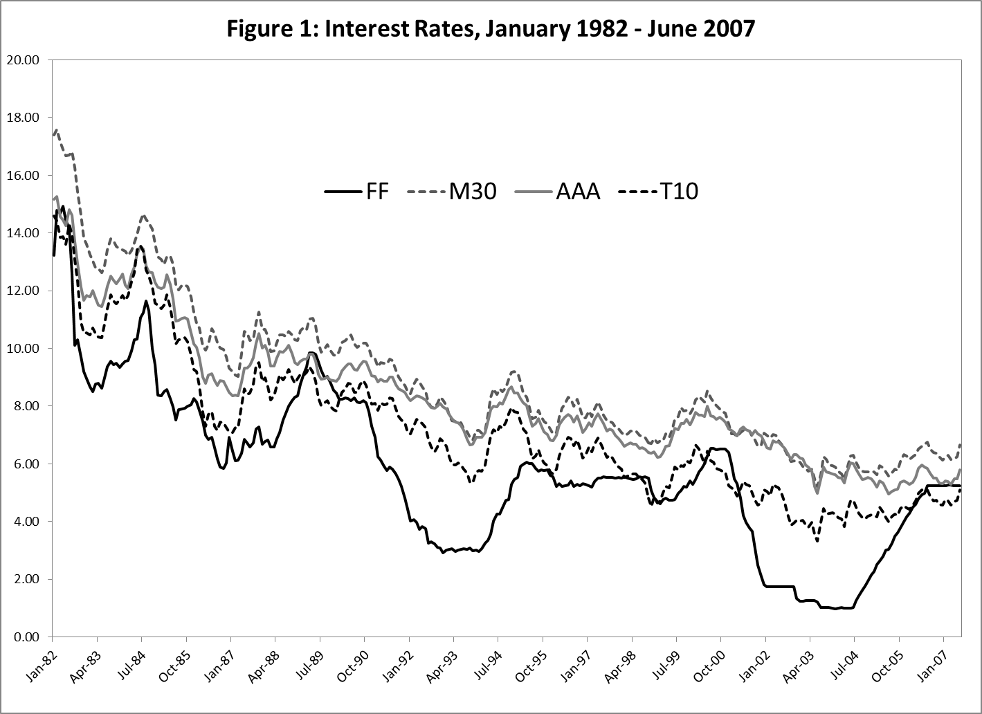
The strong correlation between the funds rate and other rates shown in Figure 1 might give one the impression that the Fed exerts considerable control over a broad range of rates. But this is an artifact of the common downward trend in rate, which is due in large part to the downward trend in inflation during the period and other factors. Figure 2 shows the same rates when a common quadratic time trend is removed.
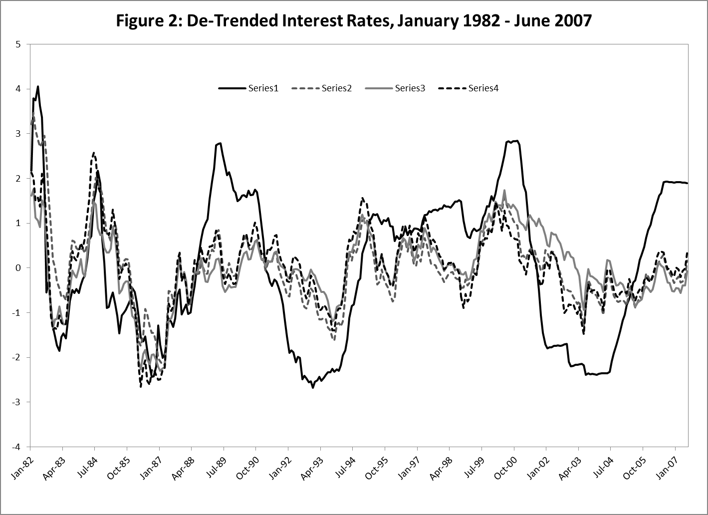
Then, all four rates move closely together until the around the middle 1990s, when the federal funds rate begins to behave much differently than the other rates. Elsewhere (Thornton 2015e), I show that this coincides with the FOMC adopting the federal funds rate as its policy instrument. Prior to the late 1980s, the funds rate moved freely with other rates. Beginning in the late 1980s, the funds rate moved only when the FOMC changed its funds rate target. This caused the relationship between the funds rate and these other rates to break down. Specifically, cyclical swings in the funds rate became enormous relative to those of the other rates and the correlation between changes in the funds rate and these rates dropped dramatically. Indeed, from June 2004 to July 2006, the FOMC increased the funds rate target from 1 percent to 5.25 percent, and the other rates barely moved—the so-called Greenspanconundrum. Changes in the federal funds rate had little effect on long-term yields, but had a larger effect on shorter-term Treasury yields.
The Phillips Curve has no empirical support: the Aggregate Supply curve is undefined.
What about the PC relationship? It is evident that PC also has essentially no empirical support. For further discussion of the empirical relevance of PC, see Boldrin (2016) and Lothian (2016) . Perhaps the most important reason for the PC relationship's failure is that, while economists and policymakers frequently talk about AD and AS, as I just did, such talk is a form of “economic gibberish.” The reason is AS doesn’t exist. Indeed, any economist worthy of the name knows this almost instinctively. AS doesn’t exist for the simple reason that producers’ supply functions can be aggregated only if all producers are operating in perfectly completive markets. If markets are oligopolistic, as nearly all markets are, one cannot even identify a firm’s supply function—a firm’s supply function doesn’t exist. If you add up a bunch of things that don’t exist, you get something that, well, doesn’t exist.[7] If AD increases relative to something that doesn’t exist, you really can’t say what might happen. This means that any talk of inflation being due to an excess of AD over AS or lack of inflation because AD is insufficient relative to AS is nonsense! Of course, this has not stopped economists and policymakers saying such things.
So what is AS? It’s a concept. An idea of what the economy’s aggregate supply function might look like if firms’ supply functions could be aggregated, that is, if it did exist. But because it doesn’t, it’s not a useful concept. Indeed, the fact that AS does not exist is the reason that GAP is not measured by the gap between AD and AS, but rather by the gap between actual and potential output.
What is potential output? It's another concept. The basic idea is that it is the amount of output the economy would produce if all the resources were “fully employed.” The concept has rather weak foundations in economic theory for a variety of reasons, not the least of which is that it is impossible to aggregate producers’ production functions. Nevertheless, economists produce estimates of it.
How? Given its weak--should I say all but nonexistent-- theatrical foundations, it's not surprising that it has been estimated in a variety of ways.[8] It is sometimes defined as “the highest level of real GDP that can be sustained over 'the long term,'” where, of course, the long term is conveniently vague. Perhaps the most commonly used estimate of potential output, is that of the Congressional Budget Office (CBO): “the level of real GDP attainable when the economy is operating at a high rate of resource use.” All of these definitions are rather fuzzy. But, of course, that’s because the concept is fuzzy, But rather than shouting, “The emperor wears no clothes,” economists continue to come up with new methods of estimating it. The goal is to find estimates of GAP (actual output less potential output) that will provide PC with empirical validity, that is, estimates of GAP that are highly positively correlated with inflation. As Boldrin (2016) says, “the thing called PC has been re-invented, re-defined and re-estimated in a different format in almost every decade since it was first 'discovered' about sixty years ago.”
The CBO estimates potential output and makes forecasts of it out to 2025Q4. These estimates and forecasts are presented in Figure 3.[9] Figure 3 also shows real GDP from 1949Q1 to 2015Q3, and an estimate of trend real GDP based on a quadratic time trend over the sample period. Note that the CBO’s estimate of potential output and the trend estimate track closely until the mid-1990s, when real GDP moves significantly above the trend line. Unlike the trend line, the CBO’s estimate of potential output increased with real GDP. The revision in the CBO’s estimate was largely due to the CBO’s belief that there was a sharp acceleration in labor productivity growth during the second half of the 1990s that continued through the 2000s (Arnold, 2009).
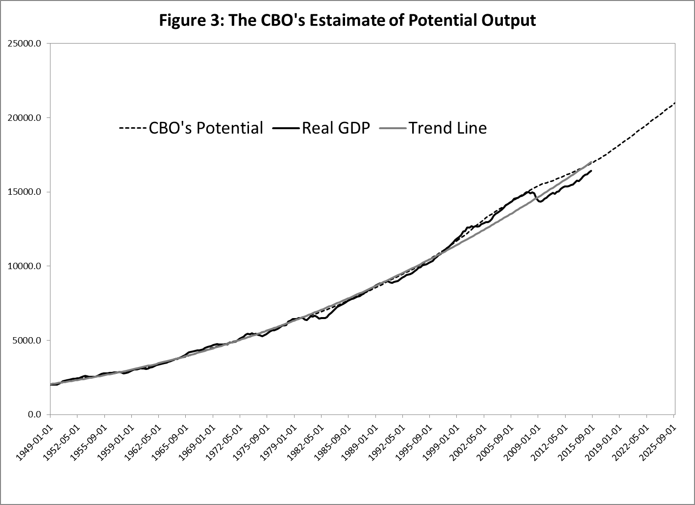
How does the CBO estimate labor productivity? Well, it doesn’t actually estimate labor productivity. Rather it estimates the growth rate of labor productivity. "How can it estimate the growth rate of labor productivity if it doesn't estimate labor productivity?” you might ask. Here’s how. First, the CBO makes an estimate of an aggregate production function. “But I thought it is impossible to aggregate firm’s production functions.” It is. But the CBO assumes that such a function exists. Not surprisingly, it chooses a specific function that has properties which economists typically attribute to a firm’s production function. It estimates this equation using total labor hours and a measure of the aggregate stock of real capital (the real dollar value of the capital stock). Specifically, it runs a regression of real GDP on total labor hours and the capital stock measure. The part of real GDP that these variables cannot account for (the residual from their regression equation) is the productivity measure, called "total factor productivity (TFP)." The growth rate of labor productivity is obtained by parsing the growth rate of TFP into its labor productivity growth and capital productivity growth components.
It is impossible to know how well a productivity measure that is derived from an aggregate production function (that, in fact, doesn’t exist) reflects actual productivity changes. Consequently, the possibility that output changed for other reasons should not (indeed, cannot) be ruled out.
Is there another explanation for the rapid growth in output from the mid-1990s to the financial crisis? Yes, a reasonable alternative explanation is that the uncharacteristically rapid growth was due to a confluence of several events, particularly advances in technology and technological innovations, the launching of the World Wide Web (1991), financial innovations (including the widespread use of securitization) and the growth of finance generally, making home ownership a national priority, and lax oversight of the mortgage and other financial markets.
The last three incentivized a boom in production of housing and ancillary products (roads and highways, appliances, trucks, heavy equipment, etc.), which dramatically increased output (think of China, whose phenomenal growth for a number of years, until recently, was largely due to a construction boom, including building ghost cities). That these factors contributed significantly to the unusually high growth during the period is evidenced by two successive asset price bubbles. The bursting of the first, the so-called dot.com bubble, caused the 2001 recession. The bursting of the second, the housing bubble, resulted in the 2007-2009 recession, which in turn brought the FOMC’s zero interest rate policy. It was hardly surprising that the 2007-2009 recession was relatively severe and long, because it was accompanied by a large overhang of real capital in the forms of residential and commercial real estate and the associated infrastructure. (There was no excess of real capital during the relatively short and mild 2001 recession.)
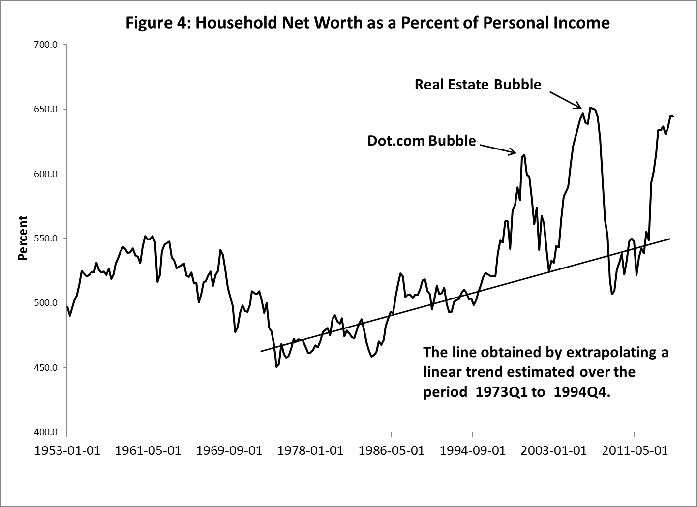
The rise in asset prices during these periods generated a historically large increase in wealth, shown in Figure 4. This increase further fueled asset prices and the production of residential and commercial real estate. The first bubble burst when investors realized that they were purchasing bad ideas; the second, when people who were purchasing houses they couldn’t afford realized that they had purchased houses they couldn’t afford. The bursting of these bubbles was, of course, associated with marked declines in wealth to levels more in line with pre-bubble behavior, but wealth is increasing dramatically again because of marked increases in both equity and house prices.
The relevant question is this: Is the historical increase in real GDP from the mid-1990s up to the financial crisis due to an abnormal increase in potential output because of a sharp rise and subsequent sharp fall in labor productivity for reasons unknown, or is it due to the confluence of several events, some of which are well known? This is difficult to answer. But whatever the answer, the period of high growth looks like an anomaly. Figure 5 shows real GDP, the CBO’s estimate of potential output, and a trend line estimated from quarterly real GDP over the period 1949Q1 through 1994Q4, just before the sharp rise in output growth. The trend line and CBO’s estimate of potential are nearly identical up to the mid-1990s. Moreover, real GDP before the mid-1990s and after mid-2009 (the end of the recession) fall nicely along the trend-line estimate of “potential.” Hence, relative to the trend line, the behavior of real GDP during the 1995-to-mid-2009 period is an anomaly.
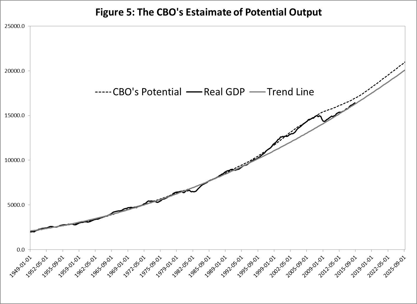
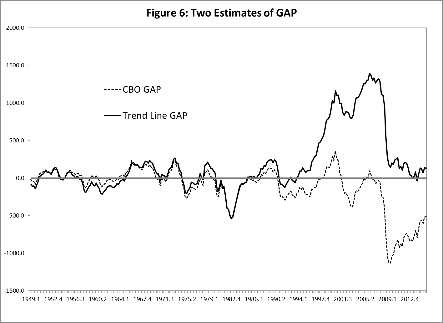
Another aspect of the CBO’s estimates of potential output, shown in Figure 5, is interesting. Its estimates of GAP have been negative (real output has been below potential) for nearly the entire period since the beginning of 1991. Indeed, the CBO’s estimate was positive for only three of the past 25 years. It seems that the economy was not operating at a “high rate of resource use,” even during most of the period when real GDP was extremely high by historical standards. This seems odd, especially since the unemployment rate was significantly lower during this period than during the two decades before 1991, when the CBO’s estimate of GAP averaged nearly zero. Figure 6 compares the CBO's estimate of the gap with a "mechanical one", based just on the trend line. Puzzling difference ...
We need better models
So why do policymakers in the U.S. and elsewhere conduct monetary policies based on a model that has so little empirical support and is theoretically flimsy? One possible reason is that beginning in the mid-1990s the FOMC has been increasingly populated by what I call “academic economists”--those who either came from academia or spent most of their careers publishing articles in academic journals. Importantly, the last two chairpersons, Ben Bernanke and Janet Yellen, are academic economists. I say "importantly" because the chairperson effectively determines monetary policy. Whatever the reason, most - but not all: the editors of this blog, among other, are part of the minority group, as is the author of this piece - (macro)economists work with the same basic model described above, and thus the model provides the language they use in talking to each other, and the foundation for their thinking about economic policy.
A puzzling question is, Why haven’t macroeconomists constructed better models of the macro economy? I believe one reason is the intuition that the aggregate economy should behave as any of its individual parts: If the price of a good increases with the demand for it, why shouldn’t the price level rise with an increase in demand for all goods? The idea is attractive and, if it were true, would make things simple. But I see no reason why one should expect this to be true. Indeed, the effect of an increase in demand on a product’s price only describes the initial effect. Higher prices induce competition (domestic and foreign) and may cause firms to move production abroad in order to reduce costs. Moreover, increased production often results in increased efficiency (what economists call economies of scale), which reduces production costs. These secondary effects tend to mitigate the longer-term effect of the increase in demand on prices and may even cause prices to be lower over a longer interval—a period of time over which most macroeconomic variables are measured.
Moreover, the economy is intrinsically dynamic. Firms continuously come into and go out of existence. So do products, which are created or destroyed by technological innovation, changing demographics, changes in tastes, or other factors. It is difficult, if not impossible, to model such dynamics in a way that matches those in the real world. Indeed, in economists’ dynamic models, the dynamics are typically based on a convenient dynamic stochastic process and a somewhat arbitrary recursive structure imposed on the model’s economic agents.
The economy is also incredibly heterogenous; which, of course, is one of the reasons AS and aggregate production functions don’t actually exist. By the way, neither does AD. In any event, it is difficult to account for such massive amounts of heterogeneity that must exist in the model’s equilibrium. Personally, I doubt that the real world has an equilibrium like the ones that exist in economic models. But if it does, it exists with a staggeringly large amount of heterogeneity.
Nevertheless, when production slows or declines, policymakers always believe it is due to a shortage of AD; perhaps because the basic model does not include any elements of production. The focus on AD is particularly odd because periods of rapid growth have been the consequence of inventions, innovations in production, and the like. The Industrial Revolution, which is credited for the first massive increase in the standard of living in history, was largely due to a revolution in production technology and major advances in chemistry, not to an exogenous massive increase in “aggregate demand.” Electricity, autos, planes, television, and cellular phones are but a few examples of products that weren’t in demand until they were produced, and whose production was accompanied by high rates of economic growth. Hence, there is no reason to believe that production will somehow begin to grow faster just because AD increased.
Indeed, while it might be difficult to understand exactly what impediments are holding back economic growth, there are strong reasons to believe that temporary increases in AD brought about by reductions in real interest rates (or in the case of fiscal policy, larger budget deficits) cannot stimulate the economy to a permanently higher level of production. Such policies' effects on output are necessarily transitory—their effect on growth nil. To understand why, consider the story that some economists want you to believe. Let’s assume that the government gives every household in the U.S. a cell phone and a 60-inch HD, smart TV at a total cost of $500 billion. To keep the story simple, we will assume that all cell phones and TVs are produced in the U.S. The story that economists tell is that output and employment in the cell phone and TV industries will rise. With more people making more, and perhaps higher, income, the demand for refrigerators, camping equipment, fingernail polish, and whatever will increase, which will further increase output and employment. This is the so-called Keynesian multiplier.
This is well and good as far as it goes, but this isn’t the end of the story. Next year the demand for cell phones and TVs will fall by $500 billion. The same “multiplier” story implies that the cell phone and TV industries will reduce production and employment. This should reduce the demand for and production of refrigerators, camping equipment, nail polish, etc., which will reduce production and employment further. There is symmetry: the multiplier must work in both directions. If the increase in demand raises output, the drop in demand must cause it to fall back to what it was before. Economists and policymakers stop their story with the first increase in output and employment. They don’t follow the story to its logical conclusion. One-off increases in demand cannot permanently raise output. This is why periods of high growth like the Industrial Revolution are driven by factors that affect production first. Demand follows along naturally. Why naturally: well, for the simple reason that when Mr. Smith becomes more productive and understands he's going have an increasing income not just tomorrow but also the day after he goes out and buys "stuff". That is how an increase in productivity of the average worker brings about an increase in demand. And when credit conditions make it possible to demand new stuff as soon as the income growth materializes, demand moves up quickly.
Then is there nothing that monetary policy can or should do to facilitate economic growth? No. Monetary policy can stabilize prices. Indeed, many economists (mostly Keynesian economists) believed that monetary policy was ineffective for controlling inflation before Paul Volker used it to end the so-called Great Inflation of the 1970s and early 1980s. Quickly--without a change in their theoretical beliefs or in the empirical evidence that led to this conclusion--all economists came to believe that inflation could be controlled by monetary policy.[10]
In addition, the Fed can also facilitate markets' natural healing process when there is a strong financial event like the financial crisis. Elsewhere (Thornton, 2014), I argued that the FOMC should have done this in the early 2008 when it became clear that the crisis, which began on August 9, 2007, was intensifying. Specially, the FOMC should have injected a massive amount of liquidity into the market through open market purchases of government securities and announced that the liquidity would be withdrawn when markets stabilized. Instead, the Fed lent funds to selected financial institutions and simultaneously offset the effect of these actions on the total amount of credit in the economy by selling an equivalent amount of government securities. The effect of these actions was predictable: the financial crisis continued to intensify.
As evidence that this policy would have been effective, I noted that after Lehman Bros announced bankruptcy on September 15, 2008, the Fed massively increased the supply of liquidity by making loans to financial institutions, and it did not offset the effect on the total supply of credit through open market sales (even though it wanted to, see Thornton, 2015a). The result was what Milton Friedman and Anna Schwartz had predicted. By early 2009, default risk spreads, which increased to extraordinary heights following Lehman’s announcement, had declined significantly and the recession, which began in November 2007, ended in June 2009. Unfortunately, the FOMC decided it could do more and engaged in a bond-buying binge called quantitative easing (QE).[11]
Unless, there is a fundamental change in the model used for making policy, I see no way the FOMC will change its approach to conducting monetary policy. The recent relatively large reductions in asset prices and signs of a marked slowing in global economic growth will likely cause the FOMC to postpone further increases in its target for the funds rate. Indeed, if the FOMC becomes concerned that the U.S. may be heading for another recession, it will likely purchase even larger amounts of securities, reduce the target back to zero, or perhaps even charge banks an interest rate of 25 to 50 to hold excess reserves. In short, the FOMC will pursue the same policy and expect different results—I call this monetary policy insanity (Thornton, 2015c).
References:
Arnold, R.W. (2009). “The Challenges of Estimating Potential Output in Real Time,” Federal Reserve Bank of St. Louis Review, 91(4), 271-90.
Bernanke, B.S., and M. Gertler. (1995). “Inside the Black Box: The Credit Channel of Monetary Policy Transmission,” Journal of Economic Perspectives, 9(4), 27-48.
Boldrin, M. (2016), "Comment on 'A Wedge in the Dual Mandate' ....,", Journal of Macroeconomics 47(Part A), 26-32.
Borio, C., P. Disyatat, and M. Juselius. (2014). “A Parsimonious Approach to Incorporating Economic Information in Measures of Potential Output,” BIS Working Paper, No. 442.
Bryson, B. (2003). A Short History of Nearly Everything, Broadway Books.
Campbell, J., and N.G. Mankiw. (1989). Consumption, Income, and Interest Rates: Reinterpreting the Time Series Evidence, with John Campbell, NBER Macroeconomics Annual 4, 1989, 185-216.
Cerra, V. and S.C. Saxena. (2000). “Alternative Methods of Estimating Potential Output and the Output Gap: An Application to Sweden,” IMF Working Paper, March 2000.
Garratt, P., K. Lee, E. Mise, and K. Shields. (2008). “Real-Time Representations of the Output Gap,” The Review of Economics and Statistics, 90(4), 792-804.
Howitt, P. (1990). “Zero Inflation as a Long-Term Target for Monetary Policy,” in Zero Inflation: The Goal of Price Stability, Richard G. Lipsey, ed. C. D. Howe Institute, 1990.
Lothian, J (2016), "Comment on Rudebusch and Williams ...," Journal of Macroeconomics, 47(Part A), 19-25.
Marty, A.L. and D.L. Thornton. (1995). “Is There a Case for “Moderate Inflation?” Federal Reserve Bank of St. Louis, Review, 77(4), 27-38.
Sharpe, S.A., and G.A. Suarez. (2014). “The Insensitivity of Investment to Interest Rates: Evidence from a Survey of CFOs,” Finance and Economics Discussion Series 2014-02, Divisions of Research & Statistics and Monetary Affairs, Federal Reserve Board.
Thornton, D.L. (1996). “The Costs and Benefits of Price Stability: An Assessment of Howitt’s Rule,” Federal Reserve Bank of St. Louis, Review, 78(2), 23-38.
Thornton, D.L. (2010). “How Did We Get To Inflation Targeting And Where Do We Go Now? A Perspective From The U.S. Experience,” Inflation Targeting Twenty Years On: Past Lessons and Future Prospects. David Cobham, Øyvind Eitrheim, Stefan Gerlach and Jan Qvigstad, (ed.) Cambridge University Press, pp. 90-110.
Thornton, D.L. (2012). “The Dual Mandate: Has the Fed Changed Its Objective?” Federal Reserve Bank of St. Louis Review, 94(2), 117-134.
Thornton, D.L. (2014a). “The Federal Reserve’s Response to the Financial Crisis: What It Did and What It Should Have Done.” In Chadha, Durre, Joyce, and Sarno ed. Developments in Macro-Finance Yield Curve Modelling, Cambridge University Press, Cambridge, U.K.
Thornton, D.L. (2014b). “Monetary Policy: Why Money Matters, and Interest Rates Don’t,” Journal of Macroeconomics, 40, June, 2014, 202-13.
Thornton, D.L. (2015a). “Requiem for QE,” Policy Analysis, No. 783, November 17, 2015, Cato Institute, Washington D.C.
Thornton, D.L. (2015b). “Does Aggregate Supply Exist? Should We Care?” Common Sense Economics, Vol. 1, No. 2. at www.dlthornton.com.
Thornton, D.L. (2015c). “Monetary Policy Insanity,” Common Sense Economics Perspective,” Vol. 1, No. 8, at www.dlthornton.com.
Thornton, D.L. (2015d). “What’s the Connection between the “Rain Man” and LIBOR Rates, and the Fed’s Ability to Control Interest Rates?" Common Sense Economics Perspective, No. 9, 2015 at www.dlthornton.com.
Thornton, D.L. (2015e) “Greenspan’s Conundrum and the Fed’s Ability to Affect Long-Term Yields,” unpublished manuscript, which can be found at www.dlthornton.com.
Weber, W. (1970). “The Effect of Interest Rates on Aggregate Consumption,” American Economic Review, 60(4), 591-600.
[1] See Thornton (2012) for a discussion of how this idea came about and how it changed under Chairman Bernanke.
[2] Howitt (1990). Elsewhere (see Thornton, 1996) I show that Howitt’s Rule requires some very stringent conditions that are unlikely to hold.
[3] Bernanke and Gertler (1995), p. 27. According to the credit channel increases in interest rates reduce the value of bonds which are used as collateral for loans, making it more difficult for small businesses to obtained loans. The fact that the credit channel has gotten little support empirically is evidenced by the fact that Bernanke never cites it in his discussions of the FOMC’s zero interest rate policy.
[4] Bryson (2003) shows that in physical scientists routinely ignored facts that don’t fit well with their models, so I guess I should not be surprised that economists do it too.
[6] For a discussion of the Fed’s ability (or, more correctly, inability) to affect interest rates, see Thornton (2014b, 2015d).
[7] There are other reasons AS does not exist, but this reason is sufficient. For some other reasons, see Thornton (2015b).
Wow